Splay Trees
We learned about three types of Binary Search Tree (BST) data structures: AVL, Red-Black, and B-trees. Splay trees are another type of BST data structure. While most tree data structures attempt to improve the worst-case time per operation, splay trees follow a different approach. The splaying operation improves time for a set of m consecutive operations on a splay tree. It takes at most O(m log n) time for m consecutive operation, where n is the number of nodes in the tree. It does not preclude the case that a single operation may take up to O(n) time. So, the bound depends on the possibility of not having operations that always access the deepest leaf. It works on the premise that good and bad operations are equally likely. Some operations may be bad, but others are good. Since m consecutive operations take time of O(m log n), the amortized cost per operation is O(log n).
Splay tree works on the principle that the worst-case time of O(n) for an operation on a tree data structure is not that bad if it occurs infrequently. Such a bad operation makes the tree bushy. Therefore, the time for subsequent operations improves. For example, we may have a worst-case search in a binary search if the searched element is not present in the list. If every time the middle element is greater than the input element, then we continue to divide the tree. So, we have to perform partition repeatedly on the left half until we reach a single element list and do not find the element. The number of subdivision of the list is log n times. However, if we are lucky, then the element may be the middle element in the first division. So, it can be located in O(1) time. Both cases are possible when we search for an element in a list.
A splay tree is a BST. In accessing an element x, we perform a sequence of splay operations that moves x to the root. The nature of a splay operation depends on the following possibilities:
- x is the left/right child of its parent.
- p is the root/non-root.
- p is the left/right child of its parent. We do not discuss the other three symmetric cases.
The three non-symmetric splay operations are:
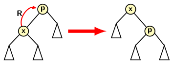
- Zig: It requires a single right (R) rotation around x.
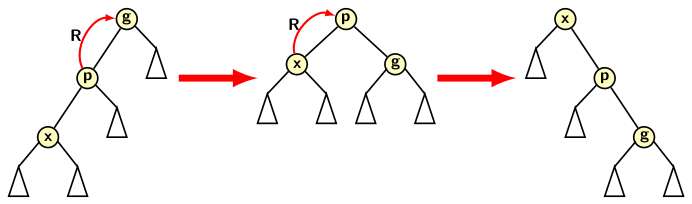
- Zig-zig: It requires a double right (RR) rotation around x.
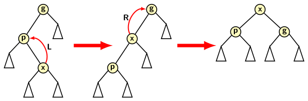
- Zig-zag: It requires a left (L) then a right (R) rotation around x.
The image below shows the three operations. The first one is a single right rotation.
A zig-zig splay is a RR type double rotation consisting of a right rotation on p followed by a right rotation on x.
A zig-zag splay is a LR type double rotation consisting of a left rotation on p followed by a right rotation on x.
Having understood the basic splay operation, let us examine how it helps using a small example is given in the image below:
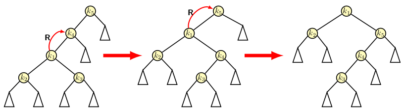
The final tree, in the bottom right most, becomes bushier than
the original tree, which appears in the top leftmost image in the above figure.
The intuitive idea behind the splay operation is that instead of applying
rotation every time, we delay the rotation until it becomes expensive.
If operations remain cheap, there is no reason to
incur extra costs for applying rotation. Only when an operation is costly,
we reorganize the tree to make future operations cheaper.
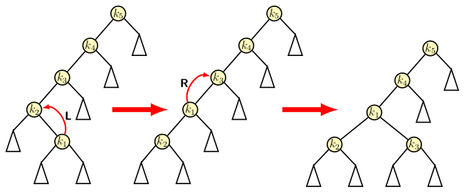
Let us see how splaying helps in an extended example. We start with an extremely skewed initial tree consisting of seven elements as in the figure below. The figure shows the initial tree in the leftmost diagram. In the description, we do not distinguish between node labels and the elements.
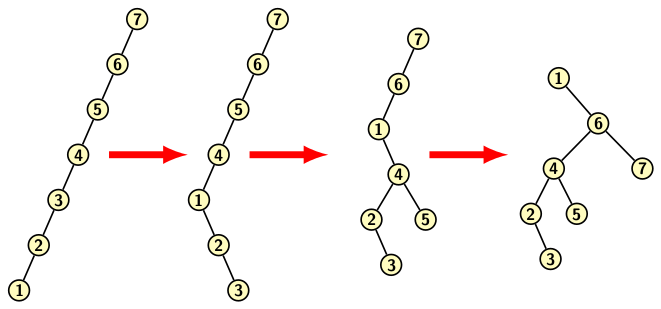
Suppose we access node 1 in the tree. After accessing
the node, we apply a sequence of splaying operations. It moves
node 1 to the root, and the tree becomes bushier than
initially. The first splay rotations start with tri-node
configuration consisting of 1-2-3. As explained earlier, it is a zig-zag pattern and
requires a double right rotation. The rotations
are as specified below:
- The first rotation brings node 3 one level down. Node 2 becomes the parent of 3.
- The second right rotation pushes node 1 to the position of 2. It becomes the parent of 2.
Since rotations preserve BST property, node 2 is the right child of 1, and node 3 is the right child of 2. Therefore we get the configuration as shown in the 2nd diagram of the figure. The second splaying operation is applied to tri-node configuration 1-4-5 of the result from the 1st splaying. Since 1-4-5 is again a zig-zig pattern and requires a double right rotation. The reader may observe that the result of 2nd splaying is shown in the 3rd diagram of the above figure. The last splay operation involves tri-node configuration 1-6-7. Therefore, applying double right rotation to it, we get the result shown in the right-most diagram.
As the reader may observe, the only rotation operations are used in turning a skewed tree into a bushy tree. Accessing node 1 takes n-1 units of time. But accessing 2 after splaying takes n/2 units of time instead of n-2 units of time. No node is as deep as it was in the original tree. However, splaying may not always lead to cheaper access to nodes. It can lead to bad reorganization of the tree when accesses are cheap.
We end this blog here.