Quick Sort Algorithm
Tony Hoare discovered the Quick sort algorithm in 1959. Like mergesort, it recursively divides the input array into smaller subarrays top-down. Each division operation divides an array into two smaller subarrays, with one subarray consisting of smaller elements than all the other subarray elements. The exchange of elements occurs during division that transfers all smaller elements to one side and all larger ones to the other. So, the algorithm belongs to the class of sorting known as the partition-exchange algorithm. The average cost of quick sort is O(n log n) for sorting of an n element array. However, the worst-case time complexity is O(n2). We will discuss the average case later in the blog.
Quick sort requires an element for the pivot that works as a fulcrum of balancing scale. The choice of pivot is critical to the performance of quicksort. If the pivot is entirely one-sided then the size of partitions becomes uneven. For example, if we choose either the first or the last element as pivot, then one subarray will consist of n-1 elements while the other will have only one element. So, the pivot should not be close to the smallest or largest element. The best choice for the pivot is the median. However, if the median finding cost is high, performance will degrade because a pivot is also needed for each subsequent partition. In our description, we assume that the input is sufficiently random. So, we neither have a sorted nor a reverse sorted sequence as input. In such a situation, we can assume the first element to be good enough for a pivot. Sometimes, we can pick the input’s first, last, and middle elements and find the median of three. Then use the median of three as a pivot. The median of three captures more randomness than using the first element as a pivot. Since the median of three takes constant time, the performance of quick sort is not affected.
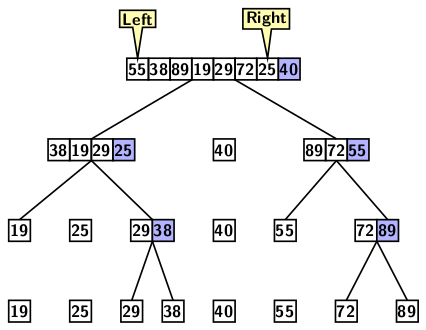
Since partitioning is the critical step, let us understand the partitioning method. We begin with a sketch assuming the first element as a pivot. As partitioning progresses, we should have the elements in sorted order.

Figure 1: Partitioning example
The figure only serves to give an insight into top-down recursive partitioning. However, it does not indicate how the partitioning method will work.
If we swap the pivot with the last element of the input array, then it shifts the pivot to position away from consideration of the partitioning of the rest of the elements. We need to divide those element into two parts:
- One set of elements S which are smaller than or equal to the pivot,
- Another set of elements G which are greater than the pivot, and
- The elements of S should occur before those of G in the array positions.
To accomplish it, we should scan over all the elements except the pivot and rearrange them in place. We create two cursors:
- The first cursor i set to one position behind the leftmost index.
- The second cursor j set to the leftmost index of the array.
Now the question is:
- How are the elements moved to create the partition?
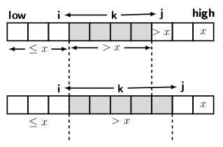
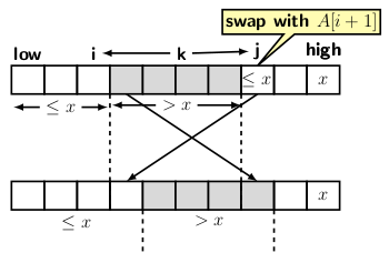
We advance both the cursors i and j as long as elements under them are smaller than pivot. Doing so ensures that none of the smaller elements are shifted unnecessarily. If the element under i + 1 becomes greater than the pivot then we stop incrementing i. At this point, we have hit the boundary for the first partition. Now we must try to expand the boundary. So, we advance j until finding an element smaller than or equal to the pivot. The two situations are depicted in Figure 2.


Figure 2: Partitioning process and its termination
The left part of the figure refers to the case when i is set at the boundary of the array with elements smaller or equal to the pivot. The cursor j continues to advance expanding the segment of the array between i + 1 and j for the elements greater than the pivot. Once we get an element smaller or equal to pivot under j, we can swap it with the element at i + 1. The swapping expands the array segments of both element types, as indicated by the right part of Figure 2. After the swapping we have to advance both i and j. The partitioning process should terminate when j has run through the array and points to the pivot’s position.
Since i points to the rightmost element smaller or equal to the pivot, all elements at index position i + 1 and beyond should be greater than the pivot. So, by swapping the pivot with the element at the index i + 1, we place the pivot at its correct position. Hence the partitioning should terminate.
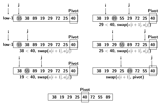
Figure 3 gives an example of partitioning. As we can find
- All elements less than or equal to the pivot occur before the elements greater than the pivot

Figure 3: Partitioning example
The algorithm for partitioning appears below.
partition(A, low, high) {
   pivot = A[high];  // Pivot
   i = low - 1 // index for smaller element
   for (j=low; j<high; j++) {
       if (A[j] < pivot) {
          i++;
          swap(A[i], A[j]);
       }
   }
   // Elements A[i+1:high] > pivot
   // Elements A[low:i] <= pivot
   swap(A[i+1], A[r]);
   return ++i;
}
The partitioning process places the pivot in the correct position. So quick sort is a straightforward recursive call to the partitioning algorithm on partitions after the pivot is in the correct position. The algorithm is given below.
quickSort(A, p, r) {
    if (p < r) {
        q = partition(A, p, r);
        quickSort(A, p, q-1);
        quickSort(A, q+1, r);
    }
}