Sorting Algorithms

We have used sorting in numerous contexts in the previous blogs. Some operations on linked lists become efficient if the lists are maintained in sorted order. Searching for an element in a list becomes efficient if the list is sorted. Binary search is applicable to a sorted list. However, we have not considered the problem of sorting in isolation. A list may be presented as a collection of elements in any order, not necessarily in sorted order. So, the question is: how do we get a sorted list in the first place? There are many sorting algorithms. We can classify them according to several characteristics.

• Based on the complexity
• Based on the number of comparisons
• Based on the number of movements
• Based on memory usage
• Based on stability
• Based on adaptability

The three measures of computational complexity are the best case, the average case, and the worst case. Since the lower bound of sorting is O(n log n) for input size of n, the best case computational complexity for sorting is O(n log n). The worst case of sorting n is O(n²). The average case is equal to the computational efforts by the sorting algorithm averaged over all possible input distributions. Typically, we consider all possible inputs equally likely and define a probability measure. We determine the computational complexity for placing the elements in sorted order using the probability measure.

Sorting is defined only as a collection of elements on which a total order is possible. A comparison between a pair of elements is the fundamental operation for finding the relative position of an element with respect to others in an input list. Therefore, the number of comparisons determines the running time of a sorting algorithm. A sorting network consists of a wired set of comparators. Counting the number of comparisons that turns an input into a sorted list gives the computation complexity. However, as we will see later, algorithms such as radix sort or counting sort do not use comparisons. So, the running time of these algorithms is not defined based on the number of comparisons.

Most comparison-based algorithms use swaps or data exchanges. In bubble sort, we move the elements to the right of the sorted section to create a vacant slot for the next element from the unsorted selection of the list. As we find, bubble sort progressively builds the sorted list from a single element to including all the elements in the input list. In radix sort the elements is placed in k bins if the radix is k in each pass.

Memory usage tells whether the algorithm requires extra (auxiliary) space for carrying out sorting operations or whether the operations are possible without any extra space. If a sorting algorithm does not require additional space, we call it an “in place” sorting algorithm.

A stable sort does not disturb the relative position of the equal elements. So equal keys maintain their relative order in the sorted list. If elements are distinct, then stability distinction is meaningless. However, some algorithms fail to maintain stability in the presence of equal elements in the input.

Adaptability influences the sorting time for some sorting algorithms. Some sorting algorithms take presortedness of the elements to reduce running time. Such algorithms are classified as adaptable.

Lower bound:

In a comparison-based sorting algorithm, for every pair of elements a_i and a_j we carry out five tests:

• a_i < a_j
• a_i ≤ a_j
• a_i == a_j
• a_i ≥ a_j
• a_i > a_j

Assuming elements are distinct, we can dispose the equality test. The remaining four test produce identical results on releative ordering. So, we just need one comparison and choose “≤” test.

Figure 1 illustrates a decision tree model for sorting three elements:

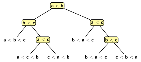
Figure 1

Every node of the decision tree model represent a comparison. The left subtree represents all subsequent comparisons when a_i ≤ a_j. Similarly, the right subtree represents all subsequent comparisons when a_i > a_j. Each leaf denotes a sorting order. So, by tracing a path from the root of the decision tree down to a leaf node we get minimum number of comparisons to reach a sorting sequence from a given input sequence. Tracing a path in decision tree amounts to finding correct permutation for sorting a list of n elements. There are n! permutations of n. So, the decision tree model with n has n! leaves. The height of the tree is log (n!). Simplifying the expression log (n!) we get:

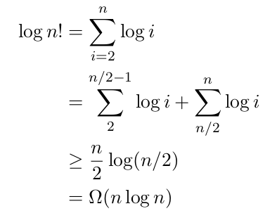
Figure 2

We will first deal with three simple algorithms:

• Bubble sort
• Insertion sort
• Selection sort

In subsequent blogs we plant to discuss a few interesting sorting algorithms such as merge sort, quick sort, and bitonic sort.

Back to Index