Introduction to Hashing
So far, we have learned about BST and balanced BSTs as possible alternative data structures for dictionary operations. As we know, insert, search and delete together constitute dictionary operations. Balanced binary search trees only ensure the worst-case time of O(log n) per operation. Dictionary operations are performed with high frequencies in a large database table application. Therefore, if an application requires a large set of dictionary operations, then even O(log n) worst-case time per operation is unacceptable. We will need a data structure that allows us to perform the operations in O(1) time on average for a given set of operations. A simple yet powerful way to store the elements in a tabular form and use the index to the table to access and retrieve them when required. The most clever part of the suggested scheme is computing the index for an element. Since the access has to be performed in O(1) time, the index should be computable in O(1) time. But the question is: how do we compute the index in O(1) time? The answer is to define the hash function.
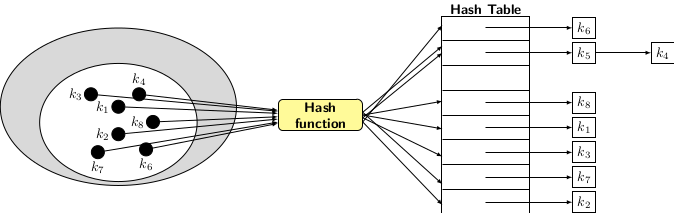
A hash function function is a mapping h:x → i, where x is element of the table and i ∈ {0, 1, 2 … }. The most challenging part of hashing is to design a hash function that spreads the elements or symbols evenly among the available table slots. How does spreading evenly help? More precisely, if more than one symbol maps to the same index, then an attempt to retrieve one specific value may produce some random value that we are not interested in. To make sense of confusion involving collisions in storing symbols in the hash table, we should know about types of hashing.
There are two types of hashing:
- Hashing by chaining
- Hashing by open addressing
Hashing by chaining uses separate linked lists to store the elements that collide on the same index value. All elements mapping to the same index are chained together in a linked list. The table index points to the first element of the list. To access the desired element, we have to traverse the linked list. The important aspect of this type of hashing is to ensure that only O(1) items may collide with the same hash value when the hash function is applied. The picture of hashing by separate chaining is given below.
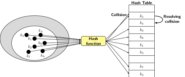
Hashing with open addressing, also known as closed hashing, uses table slots directly to store elements. There are a few collisions where the elements hash to the same table slots. There is a set of collision resolution techniques for the resolution of collisions. Some simple collision resolution techniques are linear probing, quadratic probing, or random probing. We will talk more about collision resolution techniques separately when describing closed hashing.
As explained above, hash functions are critical to the working of hash operation. We interchangeably use hash operations to mean the dictionary operations insert, search and delete. In the next blog, we discuss hash functions.