Hashing with Open Addressing
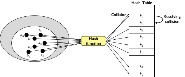
Hashing with open addressing uses table slots directly to store the elements, as indicated in the picture shown below:

The elements hashed to the same slots should be distributed to different other table slots. However, a previously hashed element may occupy the selected alternative slot. Therefore, hashing with open addressing requires a robust collision resolution technique to distribute the elements.
There are many ways to resolve collisions. We discuss some well-established collision
resolution techniques. We can view the probing function as mapping that can specify a sequencing of probes
for finding an empty slot in the table. The hash function \(h\) maps a given universe of keys \(U\) to \(m\) table slots.
$$h:U\times \{0, 1, 2, \ldots, m-1\}_{trials} \longrightarrow \{0, 1, 2, \ldots, m-1\}$$
The probe sequence is essentially a vector
$$h(k, 0), h(k,1), h(k,2), \ldots, h(k,m)$$
that is a permutation of \(\{0, 1, 2,\ldots, m-1\}\). The idea is that the probe sequence should examine all slots of the table to discover
empty slots to resolve a collision.
Linear Probing
The simplest collision resolution technique is linear probing. If a collision occurs, it tries to find the sequentially next available empty table slot. The method uses the hash function given by
$$(h(k) + i)\mod m$$.
It forms clusters of hashed elements in a few blocks of table slots. Starting with a random table slot \(x_0\in \{0, 1, \ldots, m-1\}\), linear probing
generates the probe sequence \(x_0, x_1, \ldots, x_{m-1}\), where \(x_i = (x_0 + i) \mod m\). Many of the slots may be occupied
by other elements having hash values clashing with the probes generated previously. Therefore the length of consecutive occupied slots in the table tends
to increase with linear probing. If \(j\) consecutive slots are occupied, then the probability of the next element hashing to any of
them is \(j/m\). Furthermore, if the cluster length increases to \(j+1\), the probability of another new element being hashed in one of the
previously occupied slots increases to \((j+1)/m\). It means that clusters of longer lengths tend to grow longer with more insertions.
This phenomenon is called primary clustering
Quadratic Probing
An alternative to linear probing is quadratic probing. It spreads the colliding elements by generating a probing sequence as follows. Given the first slot \(x_0\), the slot for \(i\)th probe is generated by:
$$x_i = (x_0 + ic_1 + i^2c_2)$$,
where \(i\in \{0, 1, \ldots, m-1\}\) and \(c_1\), \(c_2 \ne 0\) are constants. Quadratic probing improves performance. The distance between
successive probes in quadratic probe is determined by the sequence \(c_1 + c_2, 2c_1+4c_2, 3c_1+9c_2, \ldots\).
Let \(i\)th probe corresponding to \(k_1\) be \(x_i\) and \(j\)th probe corresponding to \(k_2\) be \(y_j\). Even if \(x_i = y_j\), with
quadratice probe \(x_{i+1}\ne y_{j+1}\). Therefore, the quadratic probe eliminates primary clustering. However, if the keys \(k_1\ne k_2\) have
the same initial hash value \(x_0\), then the quadratic probe generates an identical probe sequence. This phenomenon is known as secondary clustering.
Double Hashing
Double hashing uses two different hash functions \(h_1\) and \(h_2\). The probe sequence is generated by:
$$h(k, i) = (h_1(k) + ih_2(k))\mod m$$,
If the initial probe is at the slot position \(x_0\), then the distance between successive positions is \(h_2(k)\mod m\). Let \(h_2(k) = x_1\), then \(i\)th probe generates the slot \(x_i = (x_0 + ix_1)\mod m\) for \(i\ge 0\). The value of \(h_2(k)\) must be relatively prime to hash table size \(m\) for probing the entire table. The simplest way we can ensure it is to choose \(m\), a power of 2, and \(h_2\) to produce always an odd number. The other alternative is to let \(m\) be a prime number and design \(h_2\) to produce a positive number less than \(m\). So, we can let
\begin{array}{rcl} h_1(k) & = & k \mod m\\ h_2(k) & = & 1+ (k\mod m') \end{array}
where \(m'\) is slight less than \(m\) (it could be \(m-1\)). Each combination of the pair \(h_1\) and \(h_2\) provides \(m\) sequences. Since \(m'= m-1\), double hashing uses probe sequences of size O(\(m^2\)). Therefore, it is more random than either linear or quadratic hashing, each of which uses O(\(m\)) probe sequences. Let us consider an example where we use \(h_1(x) = x \mod 10\) and \(h_2(x) = x\mod 7\) as 7 is a prime less than 10. Suppose the insertion sequence is 67, 27, 39, 79, and 19.
- The first insertion, 67, fills slot 7.
- Now 27 cannot go to slot 7, we use the double hash to find the slot \((7 + 1\times (1+27\mod 7))\mod 10 = (7 + 7)\mod 10 = 4\).
- The third insertion hashes 39 in slot 9.
- Therefore, 79 cannot go to slot 9. Using double hash to calculate possible new position as \((9 + (1+79\mod 7))\mod 10 = 2\).
- Now, for the final insertion 19, we have a clash at slot 9 and the next slot 2. But the next probe gives \((9 + 2\times (1+19\mod 7))\mod 10 = 5\) which is not occupied. So 19 goes to slot 5.
The figure below shows the final status of the hash table using the double hashing technique to resolve collisions.

The reader can check that the choice of prime number \(7 < 10\) examines all the table slots.
In the next blog, we give an analysis of open-address hashing.