Amortised Time Complexity for Splay Trees

The contents of this blog are a bit mathematical and requires a bit of maturity in understanding. We have discussed splaying operation in a previous blog. In course of discussion we mentioned that splay tree data structure support a sequence of O(m) operations in average O(log n) units of time per operation or overall time of O(m log n). In a completely left or right skewed tree, the time for accessing the leaf node could be as expensive as O(n), where n is the number of nodes in the tree. The average time we mentioned is amortized time or time apportioned over a sequence of operations. If we consider an operation in isolation, then the average bound does not work. So, we need to provide an analysis of the amortized time.

We start with a potential function. A potential function is reserve energy, as a physicist may define it. The reserve energy tells us a system’s intrinsic capabilities to work. When we execute some activities, potentials reduce. To increase our potential, we eat nutritious food and train under a physical trainer. When performing a task, typically, we finish complex parts of the task before easy tasks. So, the remaining parts of the task become more manageable and require less energy. The amortized cost relies on a similar approach. Any expensive activity is performed in a way that makes future activities less expensive. So, the overall energy requirement for each activity is minimal.

How do we define a potential for operations on splay trees? The operations supported by splay trees normal BST operations of search, insert, and delete. These operations depend on the length of the tree path from the root to the accessed node. In the worst-case, it is equal to the height of the tree. So, we define the potential by the following function

ϕ(T) = Σlog S(i)

Where S(i) denotes the number of descendants of i (including itself). Let us define log S(i)=R(i), where R(i) is the rank (or height) of node i. Thus R(T) is the height of the tree T. We need a preliminary result for our analysis given in Lemma 1.

Lemma 1: If a + b ≤ c where a and b are both positive integers then log a + log b < 2log c - 2.

Proof: We know the arithmetic mean is less than equal to the geometric mean. So, √(ab) ≤ (a+b)/2 ≤ c/2. Taking square of both side of previous inequality, we have ab ≤ c²/4. Now take the log of both sides to get the result.

The fundamental operations for spalying are zig, zig-zig, and zig-zag. Let us focus on the complexity of these operations.

Let the ranks and sizes of a node x be denoted respectively by:

• Before splaying: R_i(x) and S_i(x)
• After splaying: R_f(x) and S_f(x)

Zig step: For completeness of description, a zig type splaying is shown in the figure below.

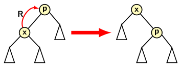
The actual time for a zig step is 1 because it is a rotation. The computation of potential change is easy. The splaying affects subtrees under x and p. The average time AT_zig is equal to the potential change for subtrees under two subtrees. Therefore,

AT_zig ≤ 1+R_f(x) + R_f(p) - R_i(x) - R_i(p)

The size of the subtree of p decreases after splaying. So we have R_f(p) < R_i(p). However, the size of subtree of x increases. So, R_f(x) > R_i(x). We can now simplify the expression for average time AT_zig for zig type splaying as follows:

AT_zig ≤ 1+R_f(x) - R_i(x)

Since R_f(x) - R_i(x) we conclude that

AT_zig ≤ 1+3(R_f(x) - R_i(x))

Zig-zag step: A zig-zig type splaying requires a double rotation, as shown in the image below.

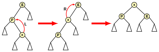
The actual time for a zig-zag is 2 (double rotation). The potential change occurs for three subtrees under x, p and g. The reader can observe that the following expression gives potential change.

2+R_f(x) + R_f(p) + R_f(g) - R_i(x) - R_i(p) - R_i(g)

From the figure we observe S_f(p) + S_f(g) < S_f(x). Therefore, from the above lemma, we can conclude: log S_f(p) + log S_f(g) < 2 log S_f(x) - 2. Since log Size = height, we have R_f(p) + R_f(g) < 2R_f(x)-2.

Summarizing the observation from the figure, we get the following:

• R_f(x) = R_i(g).
• R_i(g) > R_i(x).
• R_f(p) + R_f(g) < 2R_f(x) - 2.

Substituting R_f(g) for R_f(x), we get

2 + R_i(g) + R_f(p) + R_f(g) - R_i(x) - R_i(p) - R_i(g)
≤ 2 + R_f(p) + R_f(g) - R_i(x) - R_i(p)
≤ 2(R_f(x) - R_i(x))

Since R_f(x) - R_i(x) > 0, we have

AT_zig-zag ≤ 3(R_f(x) - R_i(x))

Zig-zig: The analysis of a zig-zag step is similar to that for a zig-zag. Amortized cost of a single zig, or zig-zag or zig-zag splay is bounded above by 3(R_f(x) - R_i(x)).

Let us examine the example of splaying given below:

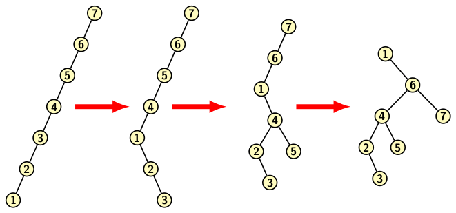
Let the four trees be denoted by T₁, T₂, T₃, and T₄ Consider the rank of node 1 in the four trees. It requires three zig-zag splays with respective costs:

• 3(R₂(1) - R₁(1)),
• 3(R₃(1) - R₂(1)), and
• 3(R₄(1) - R₃(1)).

Telescoping the sum of three expressions we get final cost as 3(R₄(1) - R₁(1)). Then we add actual access cost of the telescoped sum to get the final expression 1 + 3(R₄(1) - R₁(1)). It is of the order of O(log n). Since every operation on the splay tree requires splaying, the amortized cost of any operation on a splay tree is O(log n) where n is the number of nodes in the tree.

Back to Index